Source —
Statistics are recomputed in your browser from market data supplied by the source shown.
Educational and informational only — not financial advice, not a recommendation, and not an order.
Sign in to the Terminal
One link, no password. Your first sign-in creates a free account —
five full readings a day — every module, every timeframe.
Today's five readings are used
They reset at midnight UTC. Or keep reading now — the Pro plan removes
the limit for good.
Billed yearly it is two months cheaper. Standard covers the indicators
alone; the Terminal without a limit is part of Pro. Pay with the same
email you sign in with — your account upgrades automatically the moment
the payment completes.
Request an instrument
The Terminal opened with a small set of markets and grows where traders ask.
Tell us what you trade and we will email you the moment it is available —
nothing else, no list.
Chart key
Every line on the chart, and what it is telling you.
Price pane
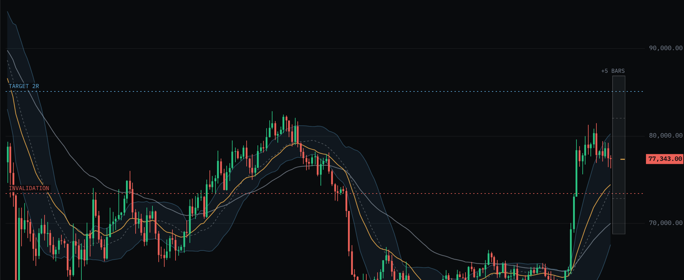
CandlesOne bar of trade — green closed higher than it opened, red closed lower.
±1σ bandThe 20-bar average ± one standard deviation. Most trade lives inside it; a close beyond it is a statistical stretch.
Band centreThe 20-bar average itself — the band's midline and the bands' anchor.
EMA 21 (amber)The fast trend line. Price holding above it means short-term pressure is up.
EMA 55 (grey)The slow trend line. EMA 21 above EMA 55 is uptrend structure; below, downtrend.
Risk frame · follows your Stop and Target settings
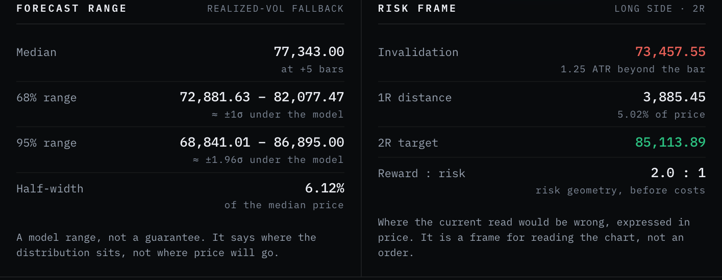
INVALIDATIONWhere the current read would be proven wrong — the Stop setting in ATR beyond the newest bar. A frame for the chart, not an order.
TARGET RThe R-multiple target: price plus the Target setting's multiple of the price-to-invalidation distance. Pure risk geometry — no support, resistance or chart structure is consulted.
Forecast box · the "+5 BARS" zone past the last candle
Model range at +5 barsWhere the model's own distribution puts price five bars ahead: the box is the 95% range, the dashed lines the tighter 68% range, and the amber mark at the right edge is the median at the horizon. “95% EXTENDS” with an arrow means that boundary continues beyond the visible price scale. The model estimates the destination, not the path. A range, never a promise.
Lower panes
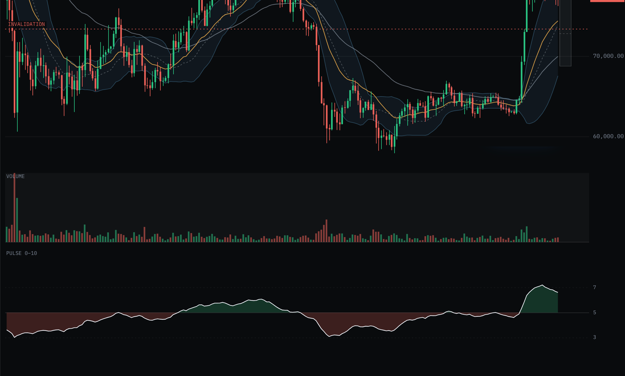
VOLUMEActivity per bar, coloured by that bar's direction — volume only means something alongside what price did with it. Some instruments (aggregate crypto and FX pairs) publish no volume: the lane says so, and Participation drops out of the setup grade.
PULSE 0–10The buying-vs-selling pressure balance. Above 5 (green) buyers lead; below 5 (red) sellers lead. 7 is the overbought line, 3 the oversold line.
The mathematics behind each element is in the
methodology section below the Terminal.
Free instrument read
Terminal
Open an instrument and read it the way the AlphaPine indicators read a chart: one blended
verdict, then the evidence behind it — bias, volatility regime, sentiment, momentum, the
conditional base rates for the next five bars, and where the read would be wrong.
Methodology
How the Terminal reads a chart
Every number on the panel is derived by one deterministic model, documented here
the way a professional terminal documents itself: each quantity defined, each
formula in its canonical form. The browser engine is public by design, so the
constants it executes — weights, windows, thresholds and decay factors — can be
inspected there. What remains proprietary is the research history and the deeper
indicator construction from which this descriptive browser model was derived.
01One payload, one model
The Terminal makes exactly one browser request per instrument and timeframe.
Its payload contains two vendor-native series: closed chart bars and closed bars
one timeframe higher. Everything on the panel — the verdict, the states, the
probabilities and the risk frame — is recomputed in your browser by one
deterministic engine. Nothing is fetched per panel: every module
is computed from the same payload, keeping the chart and the panel
internally consistent — and given the same closed bars and the same model
version, the reading reproduces exactly, on any machine, at any hour.
Only closed bars enter the model. The bar still forming is shown as the live
quote in the header, but it is excluded from every statistic: a probability
estimated on a bar that can still change is not an estimate, it is a guess
that updates against you.
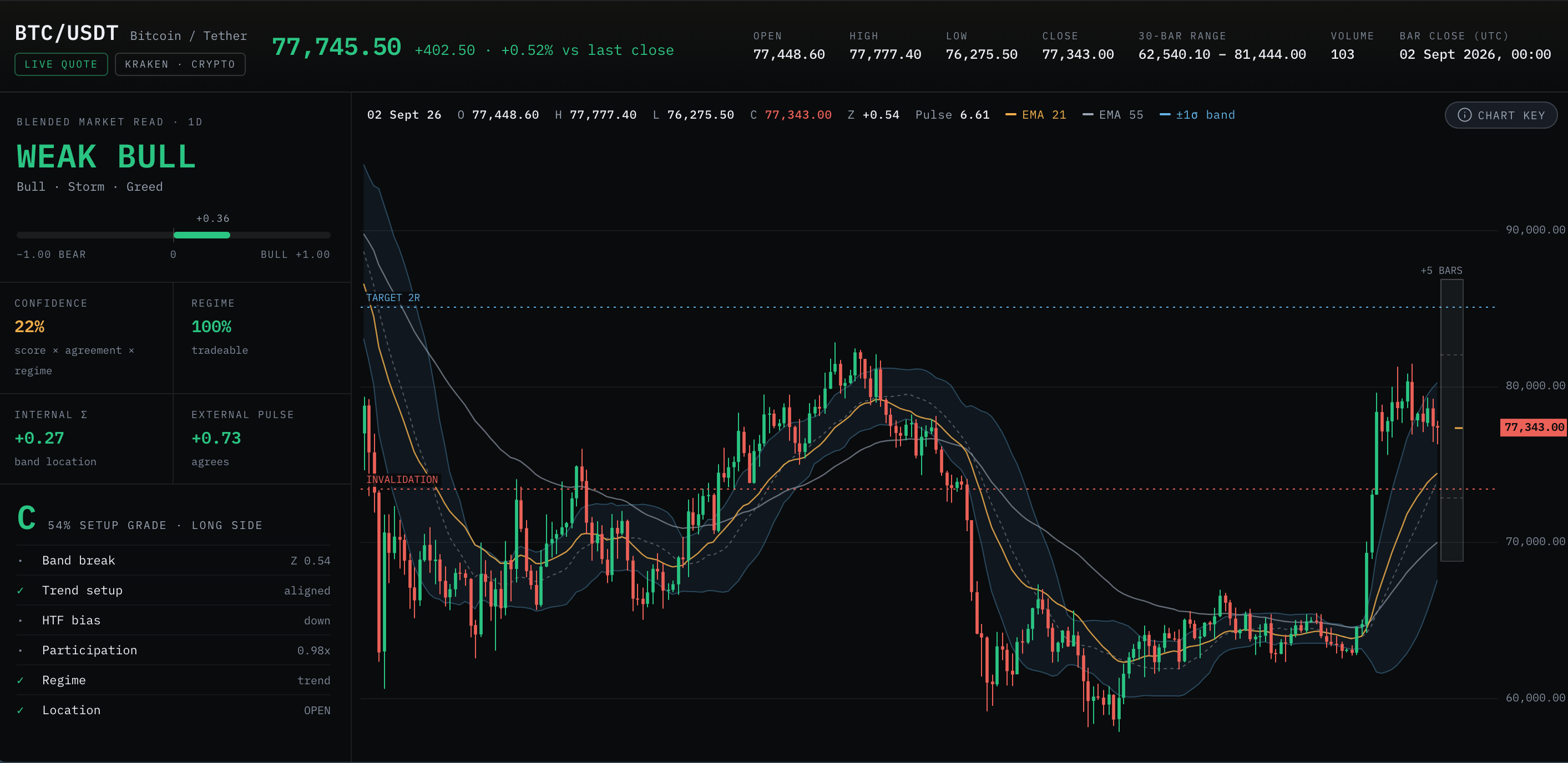
One payload carries the chart series and its native higher-timeframe context. Sample data, illustrative — not a recommendation.
02Location inside the band
The first question the model asks is where price sits relative to its own
recent behaviour. A rolling basis is taken over the 20-bar window shown in
the panel's model inputs, and the deviation of the close from that basis is
standardised into a z-score:
zt = ( Ct − μ20 ) / σ20
C = close · μ = 20-bar rolling basis · σ = 20-bar standard deviation
The σ here is the ordinary 20-bar standard deviation — deliberately. It is the
same quantity the ±1σ envelope on the chart makes visible, so the band and the
z-score can never tell two different stories, and it means the band behaves the
way a trader expects: after a violent bar the envelope widens, because the
dispersion it measures genuinely did. Where outlier-resistance matters — deciding
in step 05 whether drift is real — the model switches to a robust, median-based
scale instead, so one wild bar cannot manufacture or erase a trend. A band break
is simply |z| crossing a calibrated threshold.
Candles around the 20-bar basis (dashed) inside the ±1σ envelope — the z-score made visible.
03Pressure and trend
Two exponential moving averages — 21 and 55 bars, as shown on the chart legend
— carry the trend question. Each is the standard recursion:
EMAt = α·Pt + (1 − α)·EMAt−1, α = 2/(n+1)
the fast/slow separation, its slope, and price's side of each carry the local trend
Alongside them runs the pulse: a 0–10 oscillator, smoothed with a 3-period
Wilder average, that measures how much force the current move carries relative
to the instrument's own recent norm. Trend answers which way the tape
leans; pulse answers how hard it is leaning — and the model
treats those as separate questions, because a drifting market and a driving
market deserve different confidence even when they point the same way. How the
pulse is built from the raw series is readable in the browser engine that
computes it; the indicator suite behind it is not.
EMA 21 (amber) and EMA 55 (grey) carry the trend question; the pulse pane below scores how hard the tape leans.
04The blended verdict
The headline market score blends four legs: band location (02), the EMA
pressure balance and local trend (03), and the higher-timeframe bias read from
the vendor's last closed native bar one rung up. It is not reconstructed from
chart bars, so exchange-session boundaries remain intact. The blend is a weighted sum,
S = Σ wi · legi , S ∈ [−1, +1]
the weights wi ship inside the browser engine and can be read there; what is not published is the research and calibration history behind them
A score alone overstates itself, so it is disciplined by a confidence
multiplier: C = |S| × agreement × regime, where agreement measures
how far the internal and external legs point the same way and regime
scores whether the tape is currently tradeable at all. A strong score in a
dead tape therefore still reads as low confidence — by construction, not by
editorial judgement. The six-check setup grade beneath the verdict summarises
tactical alignment the same way; its pass conditions also ship in the browser
engine and can be inspected there.
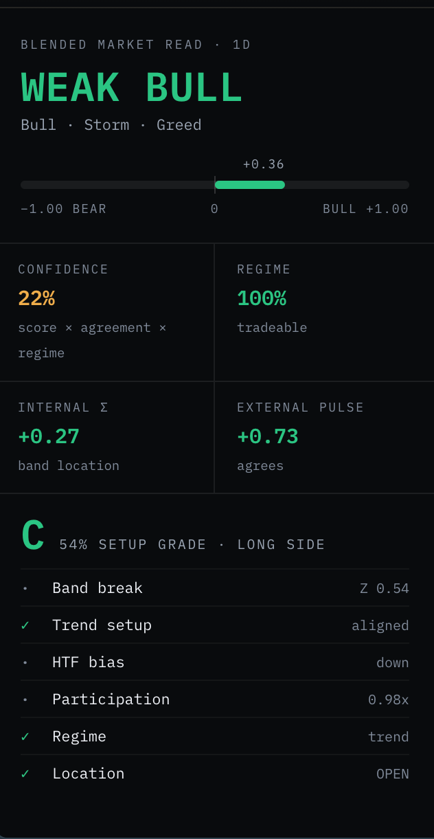
The blended read: score on its −1 to +1 meter, disciplined by confidence and regime, graded beneath.
05Eighteen market states
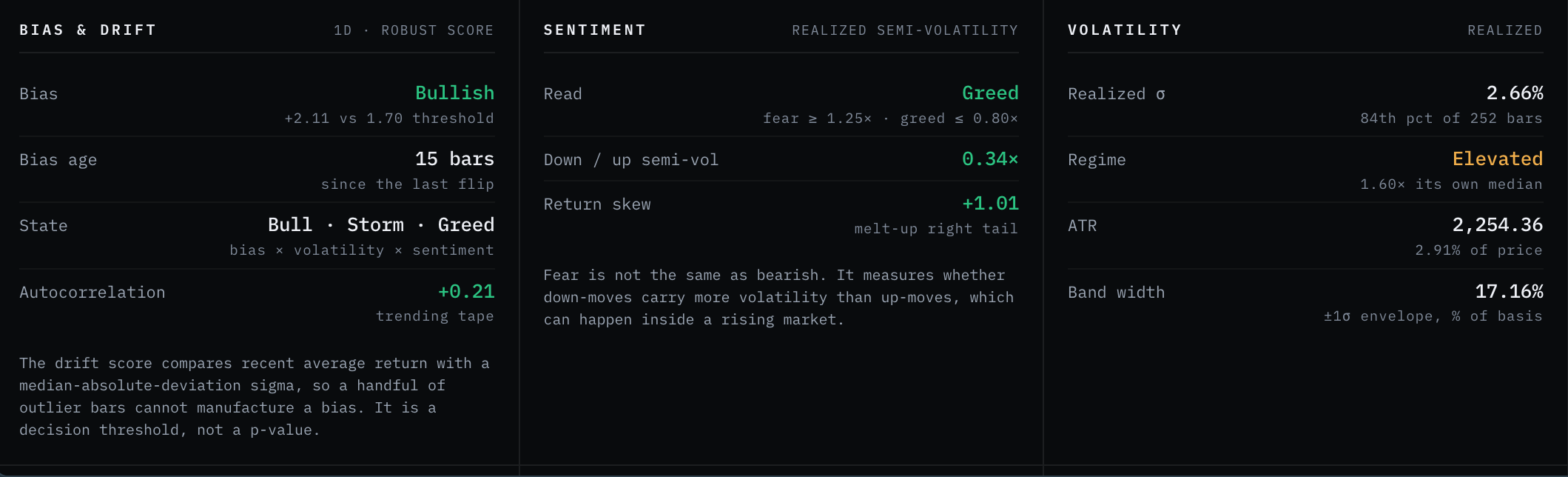
Every closed bar is placed into one of eighteen states: three grades of bias ×
three grades of volatility regime × two grades of sentiment. Bias asks whether
drift is real: mean log-return is standardised by a heavy-tail-resistant,
median-based scale — here, unlike the band of step 02, a single violent bar
must not be allowed to manufacture a trend. Volatility compares the
current dispersion with the instrument's own long-run median — an instrument
is only ever volatile relative to itself. Sentiment asks a subtler
question: whether down-moves currently carry more volatility than up-moves,
sentiment ∝ σ− / σ+
downside semi-volatility against upside — a market can rise and be fearful at once
The three questions are kept separate precisely because they disagree in the
most informative moments. The boundaries that cut each axis into its grades
are calibrated per the model. Like every constant the browser engine uses,
they can be read in it — what stays ours is how they were arrived at.
The three axes on the panel — bias × volatility × sentiment — whose grades combine into the eighteen states.
06Conditional base rates
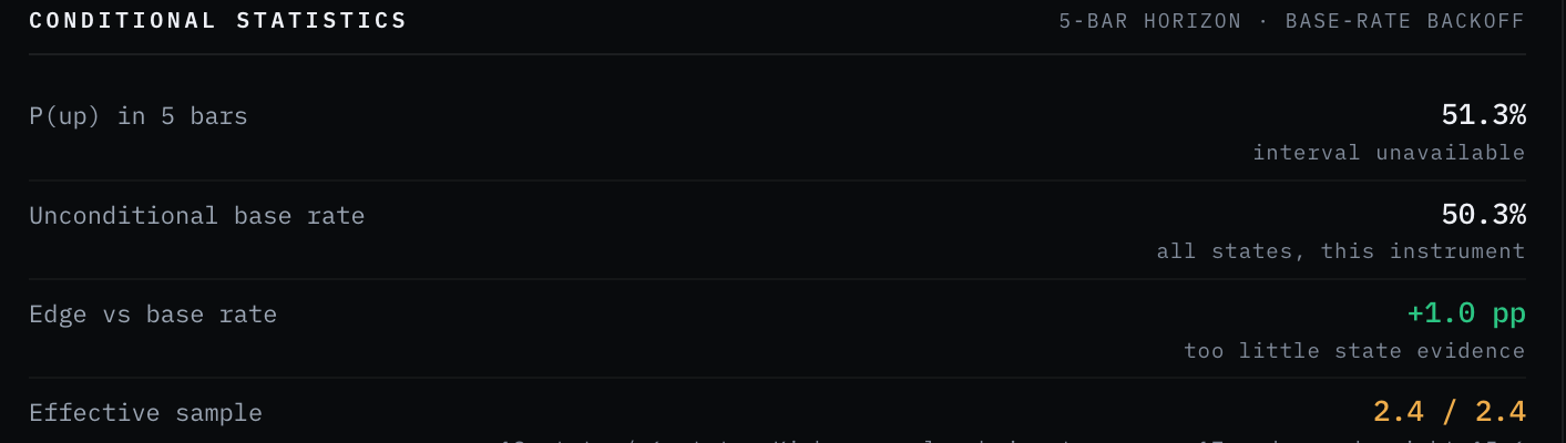
For every past bar that landed in the same state cell, the model already knows
how the next five bars resolved — the horizon shown in the model inputs. P(up)
is that historical frequency, treated with two corrections. Old regimes fade:
each observation is weighted by an exponential decay, so last year's market
votes less than last month's. And thin cells are shrunk toward the
instrument's own unconditional base rate:
This is the classical Bayesian shrinkage form; the decay constant and κ are
calibrated privately. The consequence to read off the panel: the edge
— how far p̂ sits from p0 — carries the information, not the
headline percentage. A 55% in a coin-flip instrument is a reading; a 55% in an
instrument whose base rate is 54% is noise.
P(up) is always read against the base rate — the edge row carries the information, not the headline percentage.
07Honest sample accounting
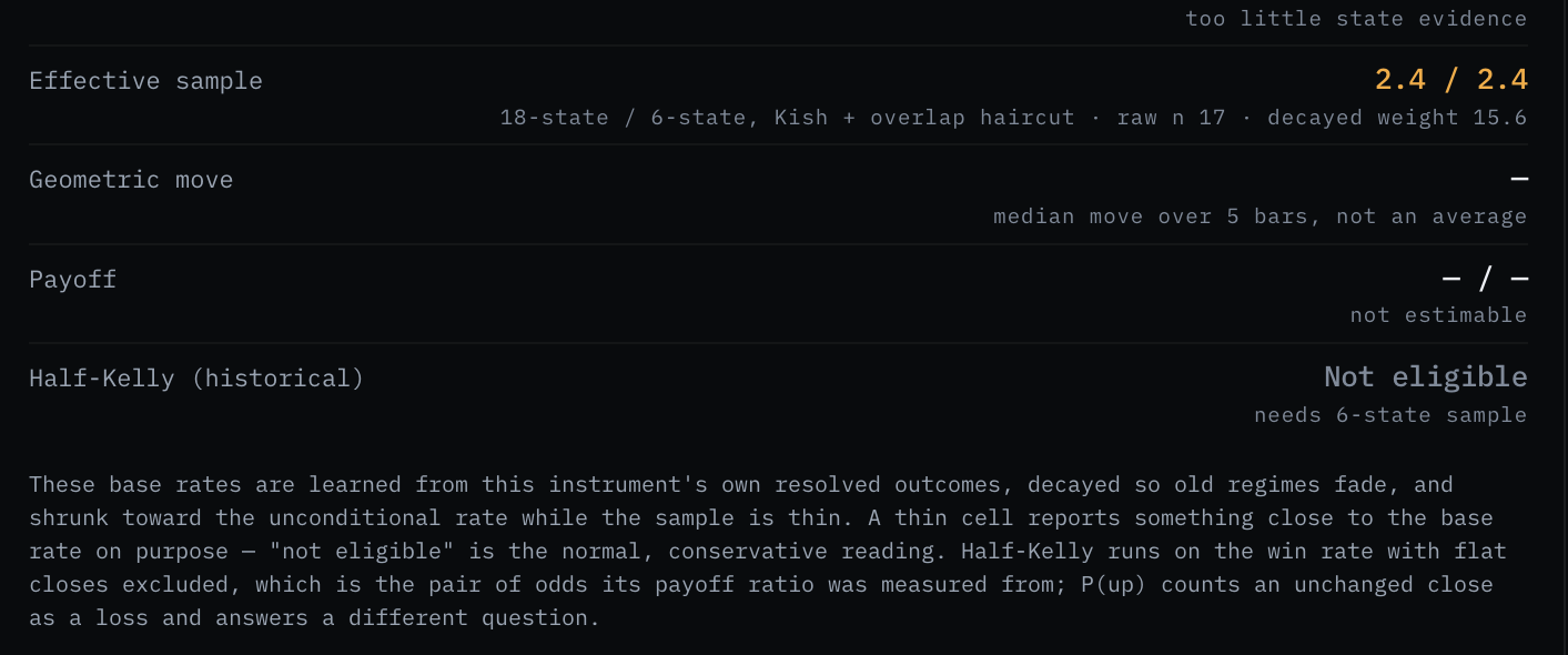
Five-bar outcomes measured on every bar overlap: consecutive observations
share four of their five bars, and autocorrelation correlates them further.
Counting them as independent would overstate the evidence several-fold, so
every quality gate in the Terminal runs on the effective sample size instead:
neff = ( Σ wt )² / Σ wt² × overlap haircut
the Kish effective-sample form, further reduced for overlapping horizons
This is why a cell showing hundreds of raw observations can still be flagged
thin, and why Not eligible is the normal reading on the sizing
module. The Terminal would rather tell you it does not know than dress a thin
sample as a statistic.
Hundreds of raw observations can still be thin after the overlap haircut — "Not eligible" is the normal, conservative reading.
08Risk frame and the ceiling
Every reading ends with the price at which it would be wrong. Invalidation is
placed a Stop-setting multiple of ATR(14) beyond the current bar's extreme
(1.25× by default), and the target at the Target setting's multiple of that
distance (2R by default) — a risk geometry that exists to make the read
falsifiable, not to tell you what to do. When, and only when, a state passes
the gates of step 07 — adequate effective sample, a 95% interval that excludes
the base rate, and a minimum count of recorded wins and losses — the panel
also shows a historical fixed-horizon half-Kelly estimate:
f* = ½ · ( p − (1 − p)/b )
p = the state's historical win rate, flat closes excluded · b = its historical
average win ÷ average loss · measured over the fixed 5-bar horizon · halved for
estimation error
Kelly is halved because estimated probabilities are not true probabilities,
and overbetting an estimate is ruin with better marketing. Two caveats are
deliberate: the estimate is historical — learned from this state's own
resolved 5-bar outcomes — and it is independent of the risk frame: changing
your Stop or Target settings reshapes the frame's levels, not this statistic,
because no simulation of your stops against the price path is performed. The
ceiling is context — an upper bound implied by the statistics — never a sizing
instruction. Nothing on this panel is financial advice; it is a measurement
system, and a measurement is only as honest as the caveats it keeps visible.
The rails frame where the read would be wrong; the +5-bar box is a distribution beside them — neither is an order.